Project 4
Overview
In the first part of this project, we implemented a more generalized morphing/warping function that allows us to rectify images and to stitch together images into mosaics. In the second part, we automated the process by which the correspondences are made when stitching together mosaics.
Project 4A
Taking Pictures
Approach
Went around the Bay to take some picture.
Results
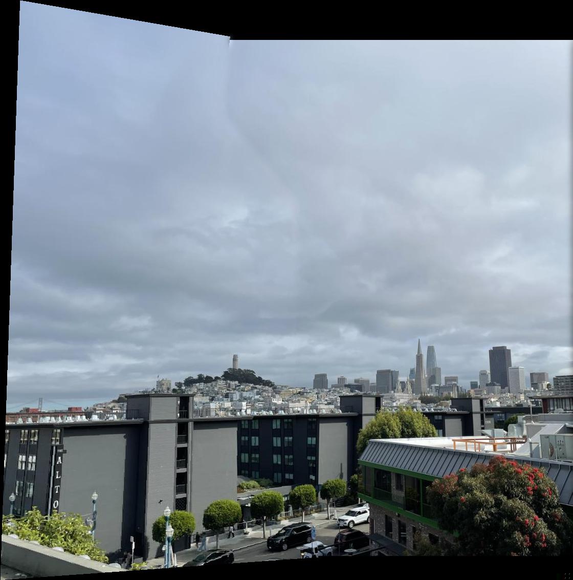
Pictures for Rectification
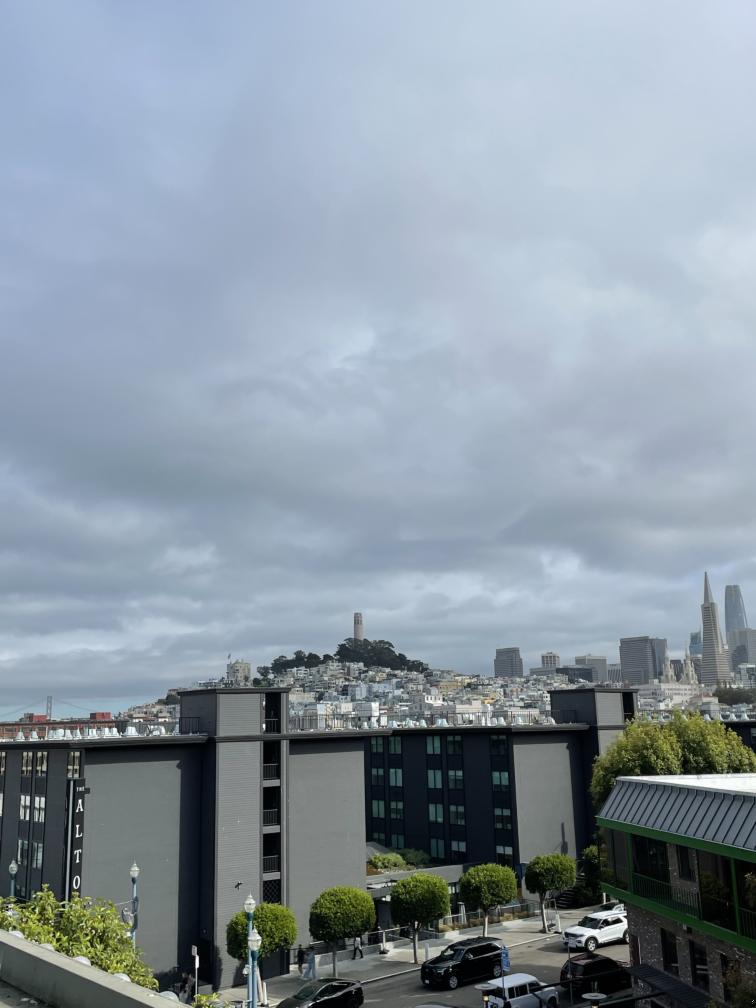
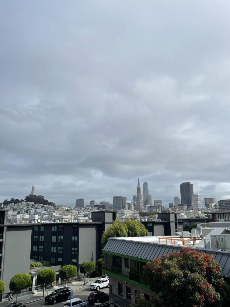
SF Skyline
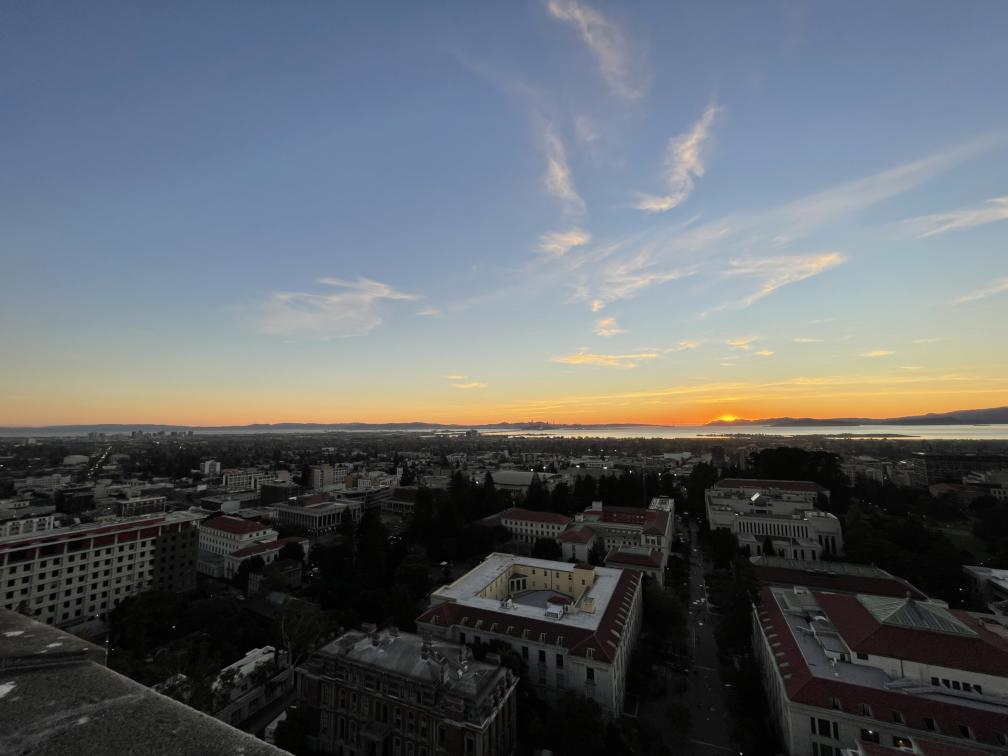
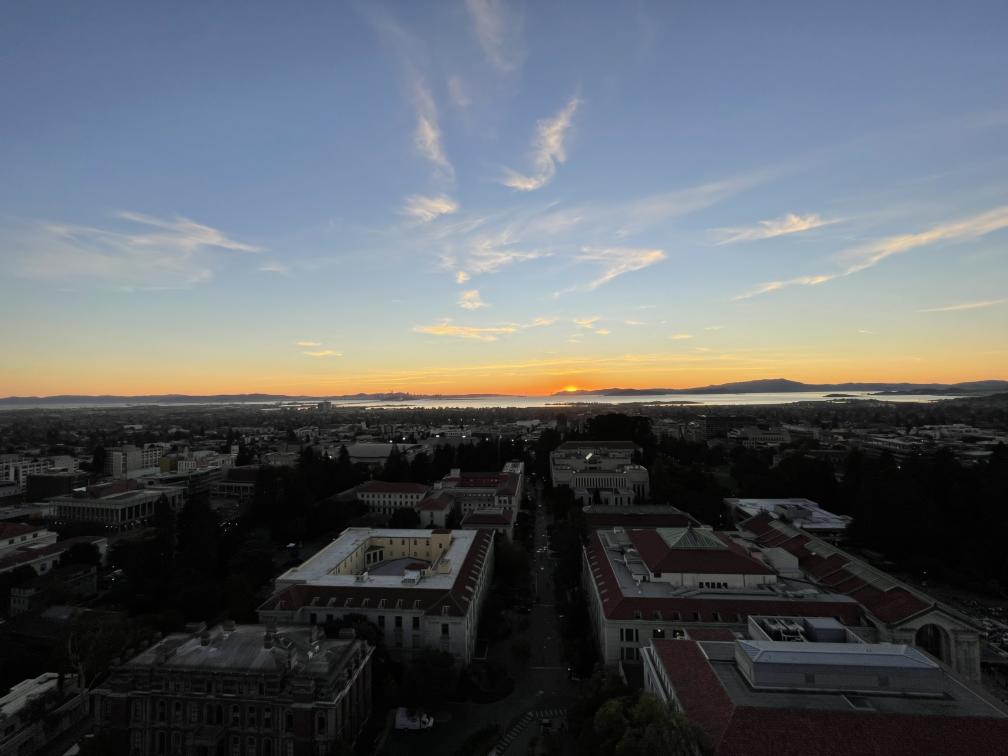
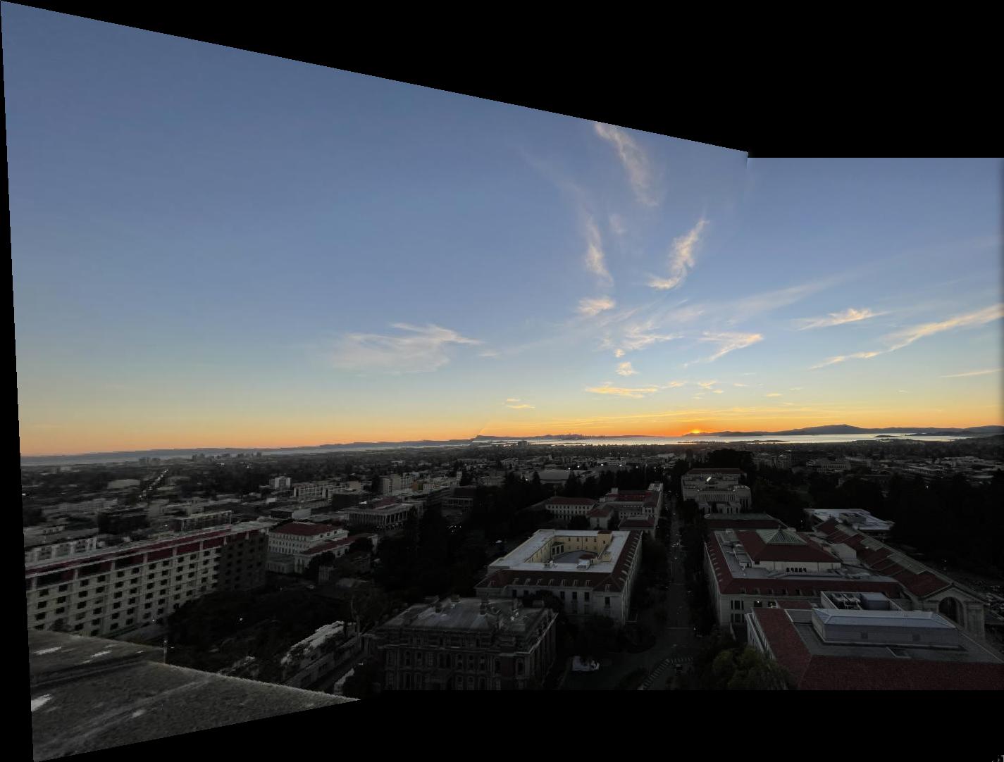
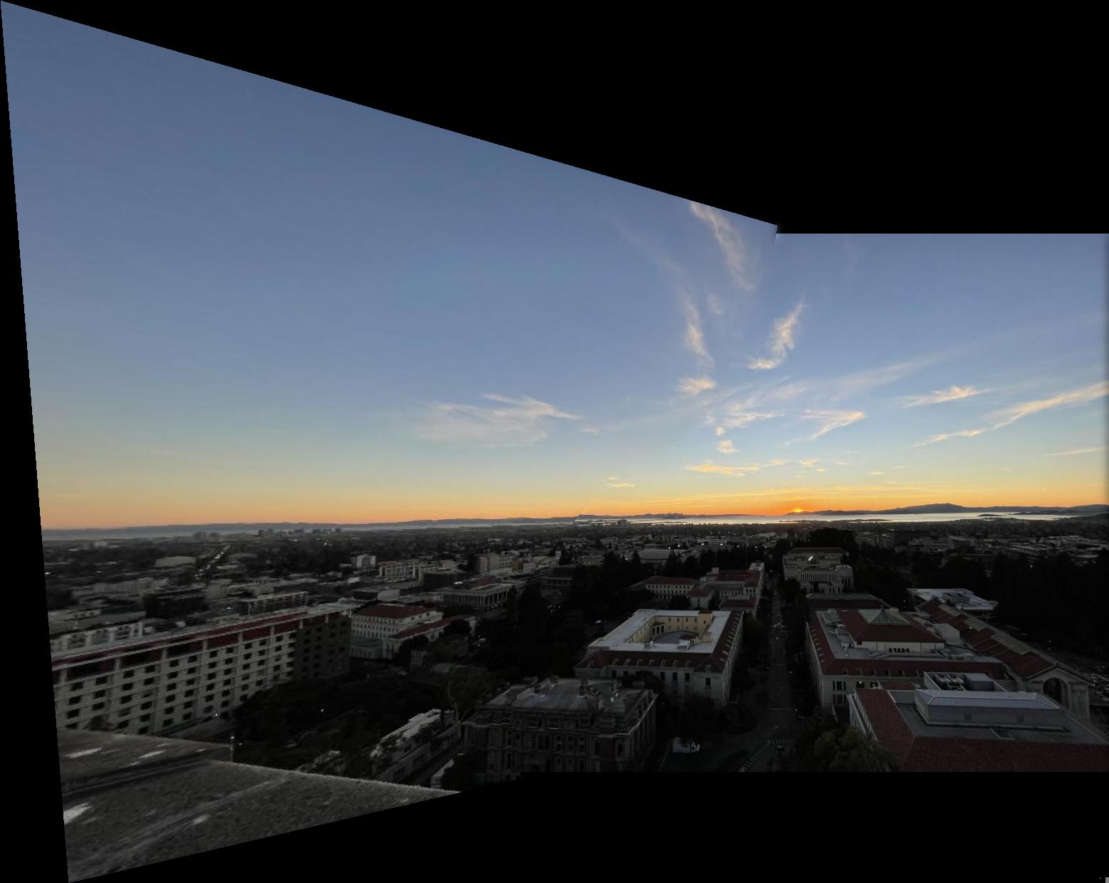
Bay Area Sunset
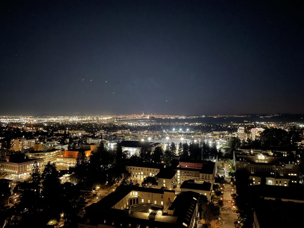
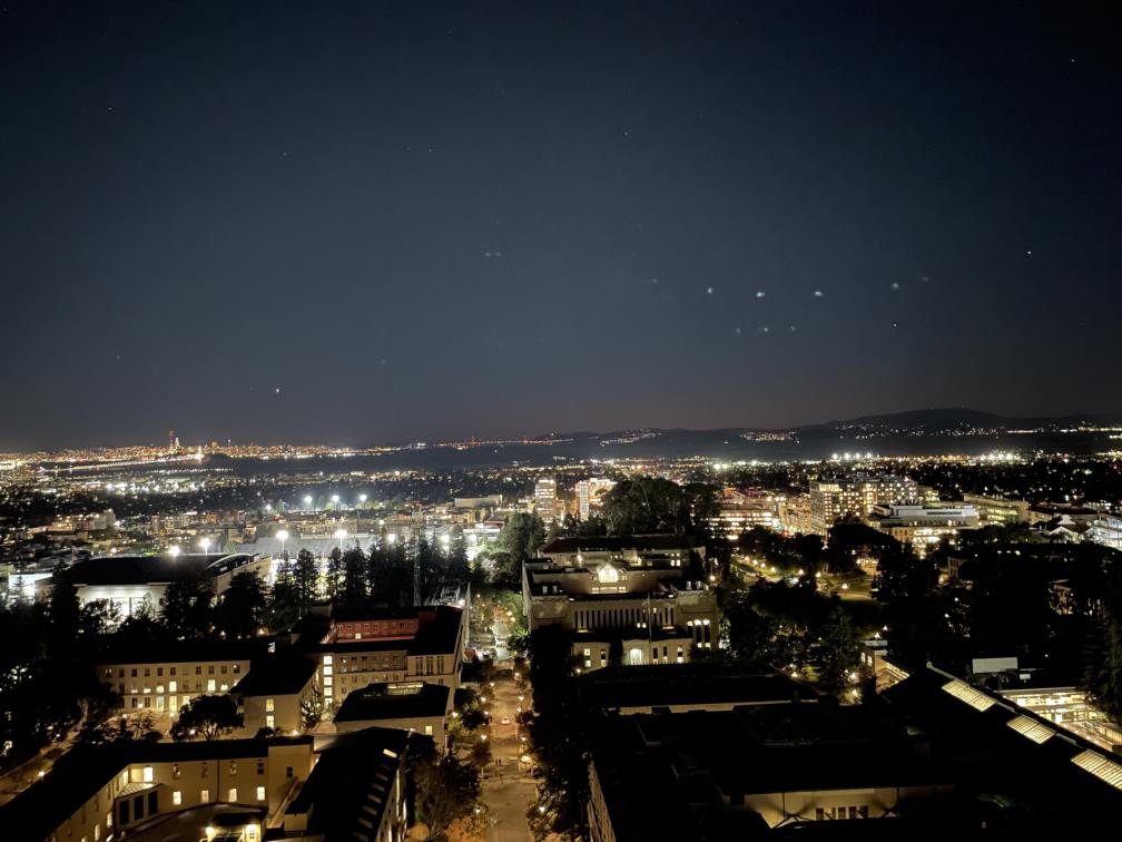
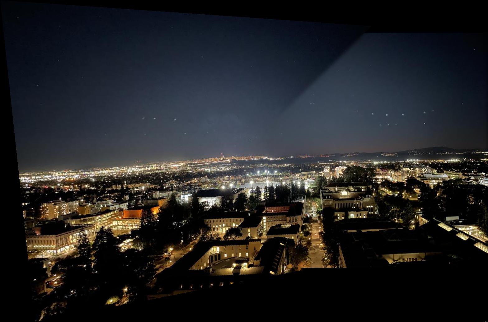
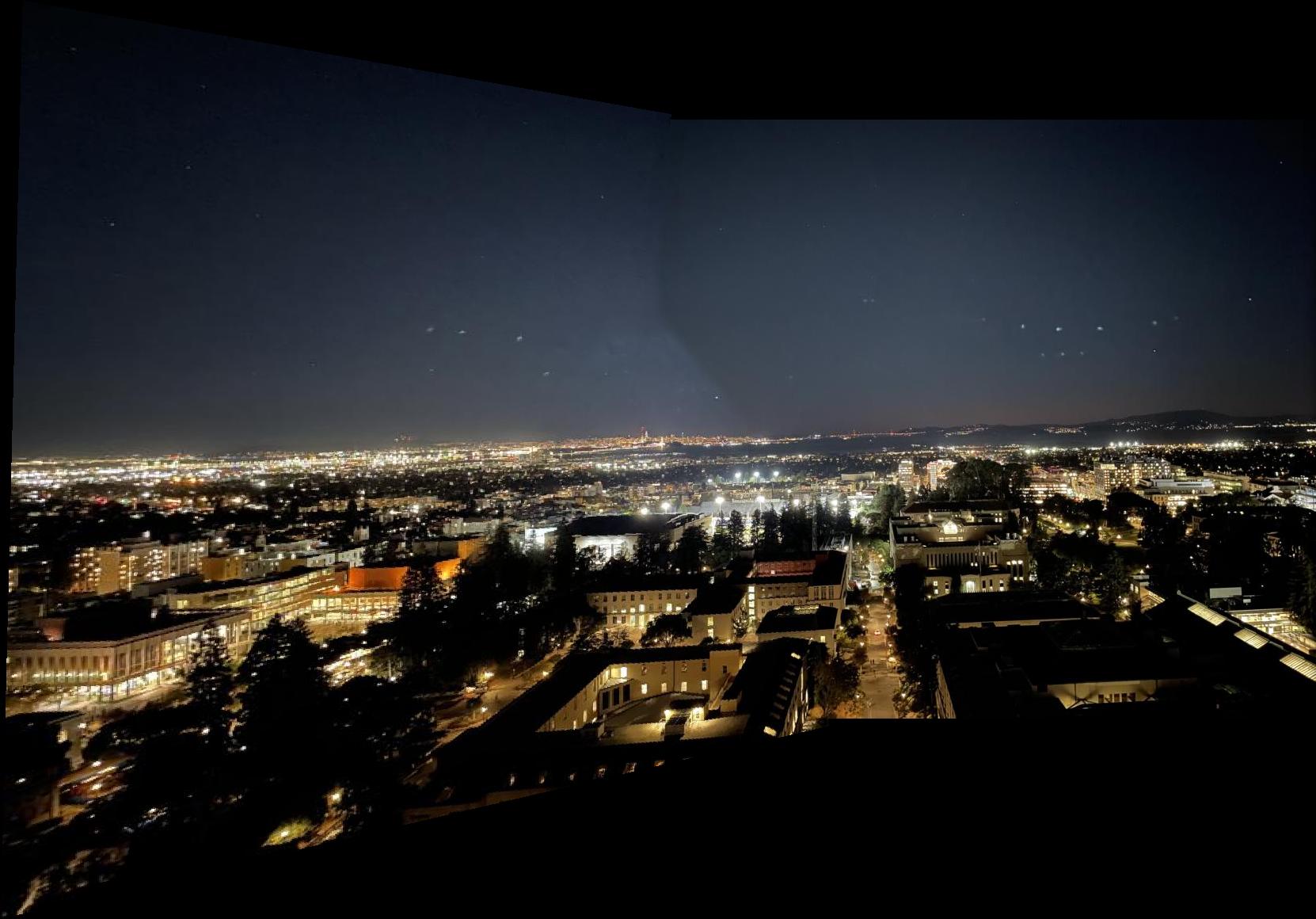
Bay Area Nighttime
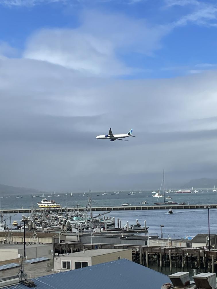
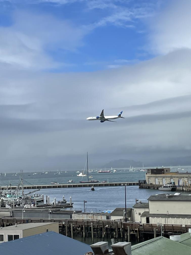
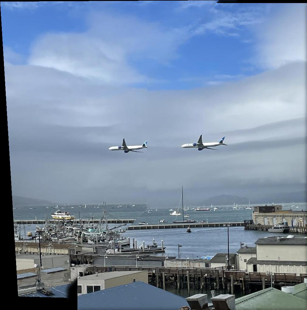
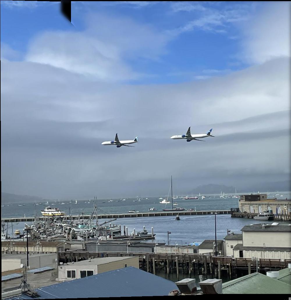
United B777 - Bay Fleet Week
Recovering Homographies
Approach
The mathematics behind the image warping that is done in this project can be described with a linear transformation called a Homography or a perspective transform. The idea is that there exists a matrix which can project the pixels of an image onto the plane of perspective of another image. This allows us to see an image from a different perspective without having to retake the image.
The Homography matrix is defined as:
\[ \begin{bmatrix}
a & b & c \\
d & e & f \\
g & h & 1
\end{bmatrix}
\begin{bmatrix} x \\ y \\ 1 \end{bmatrix}
=
\begin{bmatrix} wx' \\ wy' \\ w \end{bmatrix} \]
Namely, is is first necessary to convert the pixel indices/coordiantes into the Barycentric coordiantes by extending them to the third dimension and appending a one as the third entry. Then, if we map a pixel through \(H\), we get the corresponding pixels's indices/coordinates in the projected plane, weighted by some constant. If we divide through by the third entry and keep only the first two, we obtain the projected coordinates.
In this case, we don't know \(H\) but we do know the pixel values. This means that we can apply Least Squares to obtain the unknown coefficients in \(H\). This can be formulated as follows:
\[ \begin{align*}
&\begin{cases}
ax + by + c = wx' \\
dx + ey + f = wy' \\
gx + hy + 1 = w
\end{cases}
\\
\implies
&\begin{cases}
ax + by + c = (gx + hy + 1) x' \\
dx + ey + f = (gx + hy + 1) y'
\end{cases}
\\
\implies
&\begin{cases}
ax + by + c - gxx' - hyx' = x' \\
dx + ey + f - gxy' - hyy' = y'
\end{cases}
\\
\implies
&\begin{bmatrix}
x & y & 1 & 0 & 0 & 0 & -xx' & -yx' \\
0 & 0 & 0 & x & y & 1 & -xy' & -yy' \\
\end{bmatrix}
\begin{bmatrix} a \\ b \\ c \\ d \\ e \\ f \\ g \\ h \end{bmatrix}
=
\begin{bmatrix} x' \\ y' \end{bmatrix}
\end{align*} \]
If we repeat this process for three other pixels, we will have the necessary eight equations to solve for the eight unknowns of \(H\). Thus, we need to choose which pixels should define our Homography. This can be done by choosing specific features on the image that will be warped/projected and matching them to desired projected pixels. This part also uses this very useful website again to choose these correspondence points.
Warping Images
Approach
Once we have computed \(H\) for an image, we need to warp/project all of the pixels of that image onto the desired plane. We do this by following a very similar procedure to the one done in the previous project. However, it is not necessary to perform any triangulation for this project. Here is an overview of the procedure that I implemented:
- Map the corners of the original image through \(H\). These new pixels are the corners of the warped image.
- These projected corners might have negative values, so I create a second copy of the warped corners and align them such that the smallest entry in this list is zero. These are the shifted corners.
- Find the shape of the warped image using the warped corners: max(warped corners) - min(warped corners). Then, place the shifted corners into the skimage.draw.polygon function to get the region that our image will be projected onto.
- Remove the shift introduced in the region and perform inverse warping by mapping the entire region calculated above through \(H^{-1}\). It's necessary to remove the shift, otherwise, we don't map back to the original image correctly.
- Now that we have the pixels we want to sample at in the original image, perform interpolation using scipy.interpolate.griddata to get the value at those pixels for each color channel.
- Put everything together and place the warped image into an empty array by indexing at the polygon region.
The key in all of this is that you have to use the un-shifted version of the polygon region to obtain the corresponding sampling points in the original image. But use the shifted version of the polygon region to map into the new warped image.
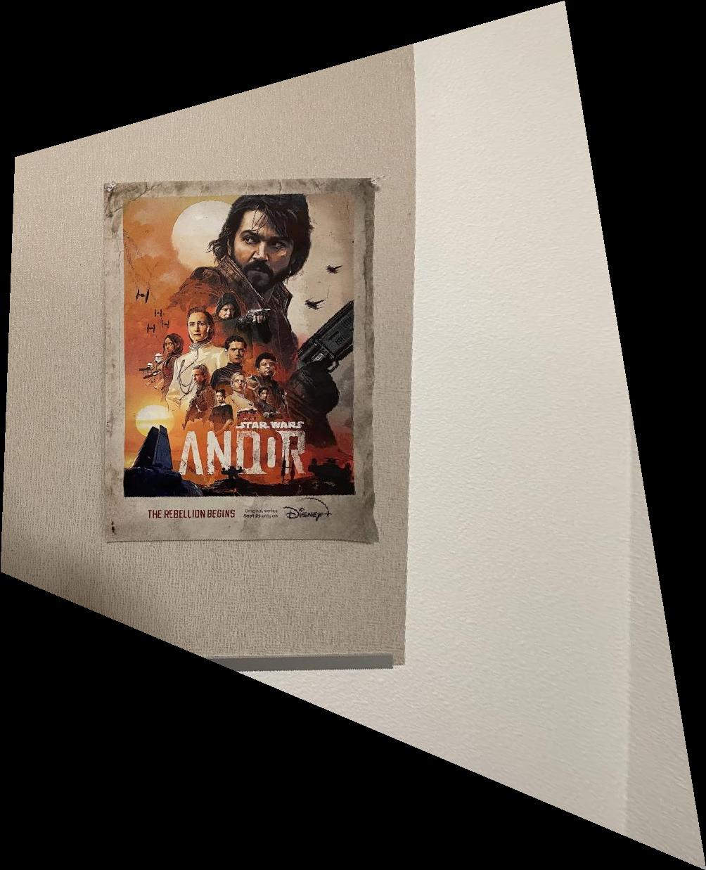
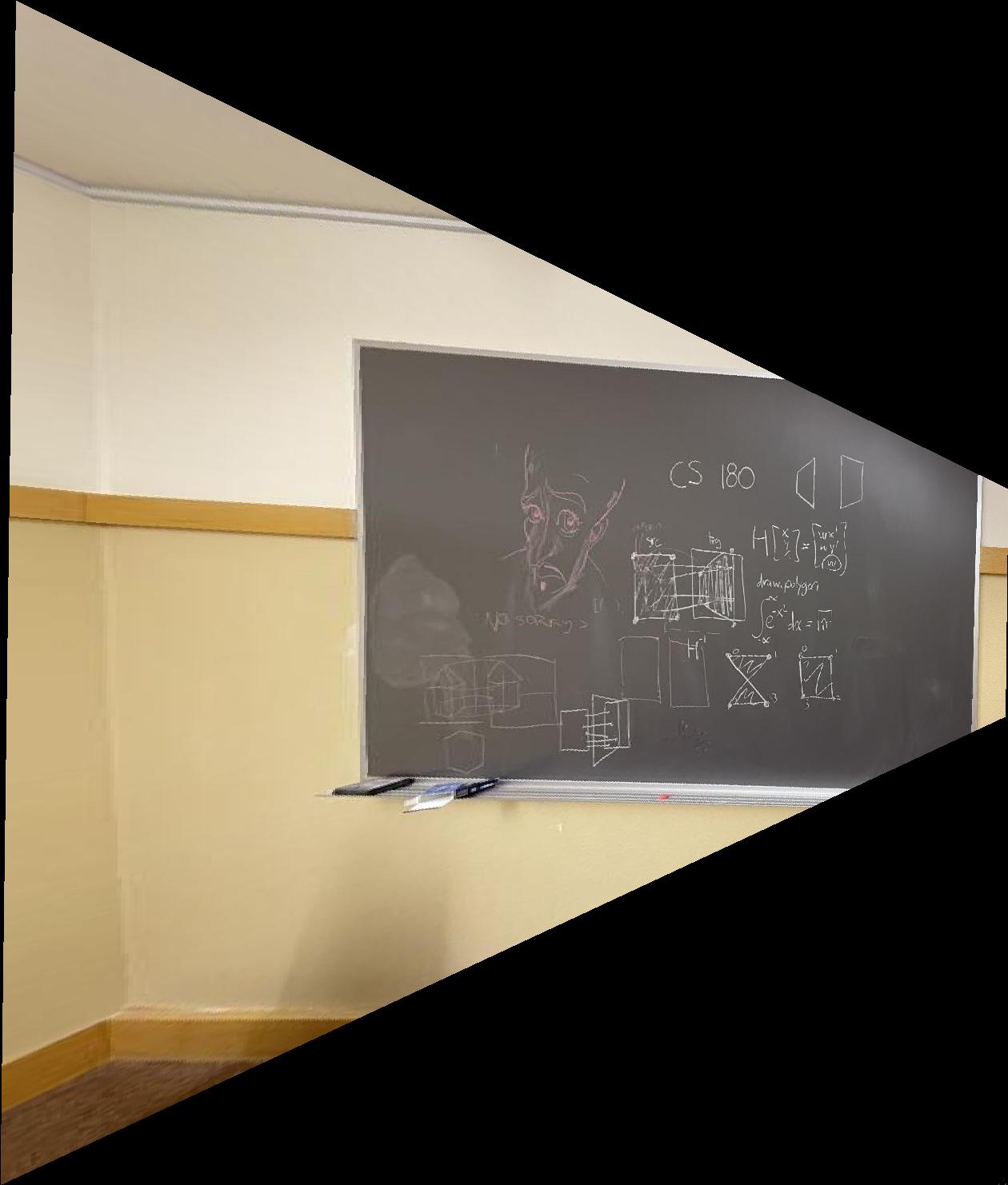
Rectified Images
Approach
Using the selected correspondences, I warp the image into a rectangle in the middle of the projected image. I compute the Homography \(H\) using these correspondences and compute the warp as described above. This procedure yielded the following results.
Results
Bells and Whistles
None for this project.
Project 4B
Harris Corners and Adaptive Non-Maximal Suppression (ANMS)
Approach
In this part, we want to find points of interest which we can use as features to automatically build the correspondences between images in a mosaic. These points of interest are called Harris corners. Using the provided starter code, the Harris corners along with their scores are calculated. Then, the ANMS algorithm allows us to suppress the vast majority of the Harris corners while maintaining a good distribution of them across the image. This is where we use the equation in the paper which introduced ANMS. The paper is titled “Multi-Image Matching using Multi-Scale Oriented Patches".
\[ r_i = \min_j |x_i - x_j| \,\,\, \text{ s.t. } \,\,\, h(x_i) < c_{\text{robust}} h(x_j) \]
Compute this for all corners \(x_i\). Then, return a desired number of best corners (I chose to return the best 300 and I also set \(c_{\text{robust}} = 0.9\)), where a corner is best if it didn't get suppressed by other corners. This ensures that the Harris corners don't clump up and are distributed evenly across the picture.
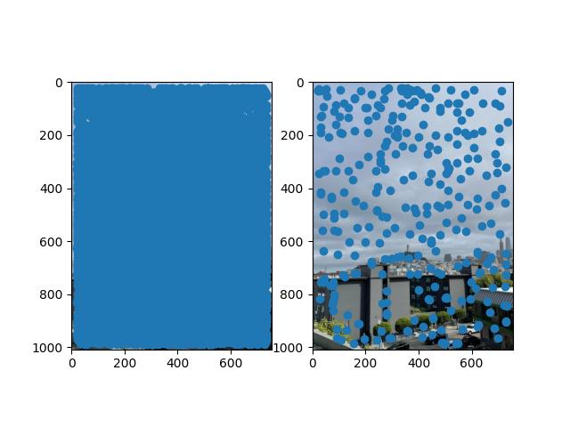
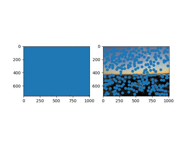
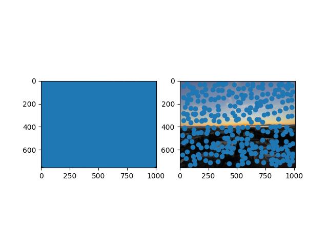
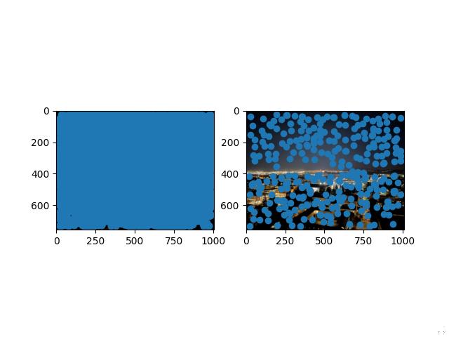
Results
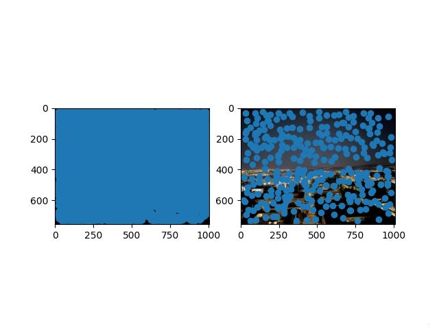
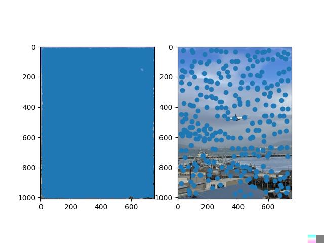
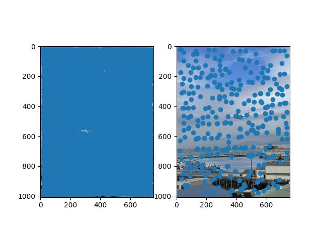
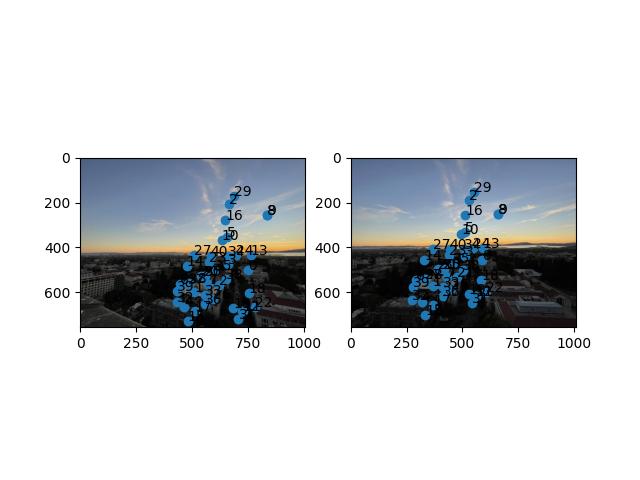
The images on the left include all of the Harris corners while the images on the right include the corners after ANMS.
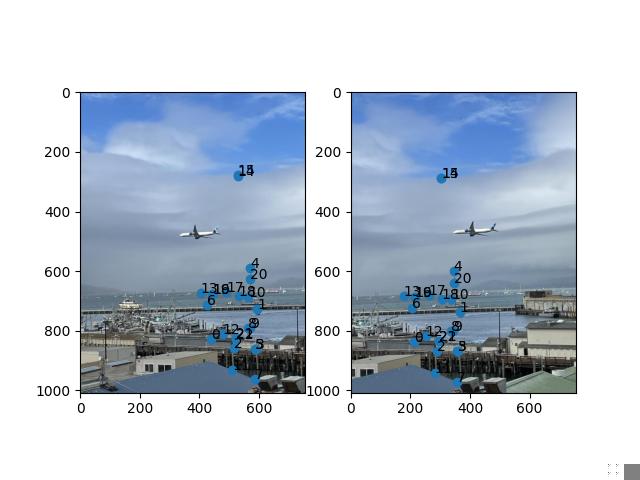
SF Skyline
Bay Area Sunset
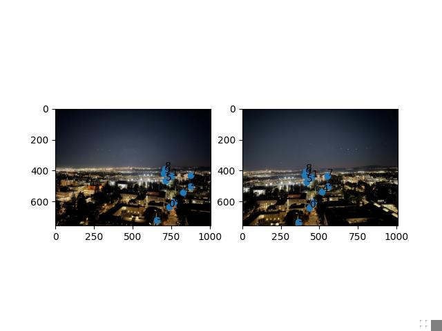
Bay Area Nighttime
United B777 - Bay Fleet Week
Feature Descriptor Extraction
Approach
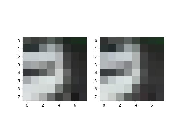
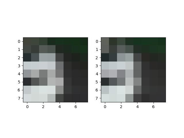
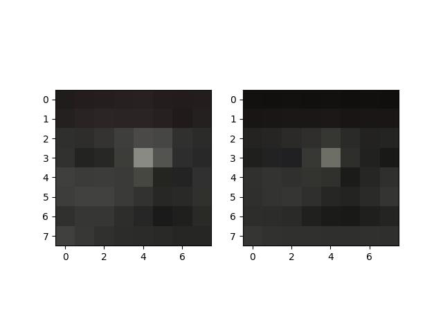
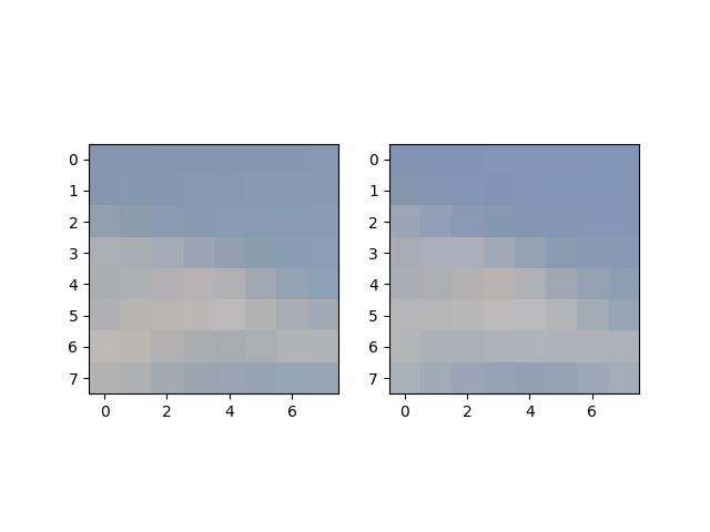
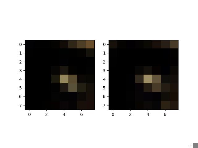
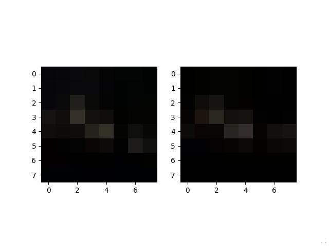
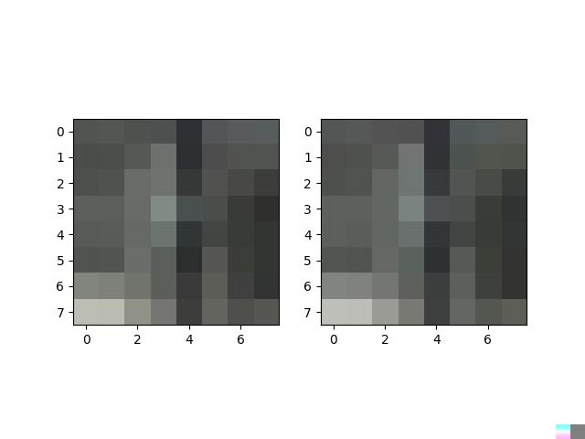
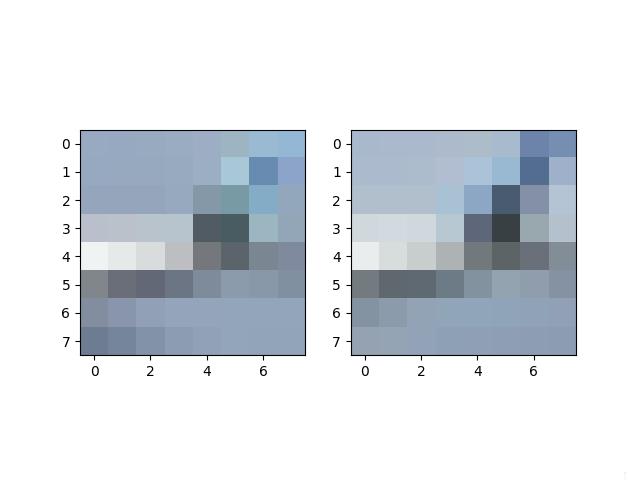
Now that we have the points of interest, we want to extract the feature that makes this point interesting. By doing this, we can reference the same features across images even if the exact pixel values are not the same. This is done by taking a 40 by 40 window from the original image centered at each ANMS corner and resizing this window to be 8 by 8. Finally, demean and divide by the standard deviation to normalize the feature. This blurs the pixel values and allows us to compare features across images.
Results
Some of the features extracted as mentioned above. Note that these are not the normalized features.
SF Skyline
Bay Area Sunset
Bay Area Nighttime
United B777 - Bay Fleet Week
Feature Matching
Approach
Now that we have the features for the images of the mosaic and the list of the corners from ANMS, we want to put everything together to obtain the matches for the corners. This is performed with Lowe's trick.
- Take the pairwise difference of all of the feature patches from the previous part. Compute the norm squared of these differences to obtain a single value for each pair of features.
- Make a copy of these values, sort them, and call these sorted values the nearest neighbors.
- Apply Lowe's trick by taking the ratio of of the 1st nearest neighbor and the 2nd nearest neighbor. If this ratio is smaller than a certain threshold (0.5), then accept a feature's match with its 1st closest neighbor. Otherwise reject it.
- Return the set of matched corners.
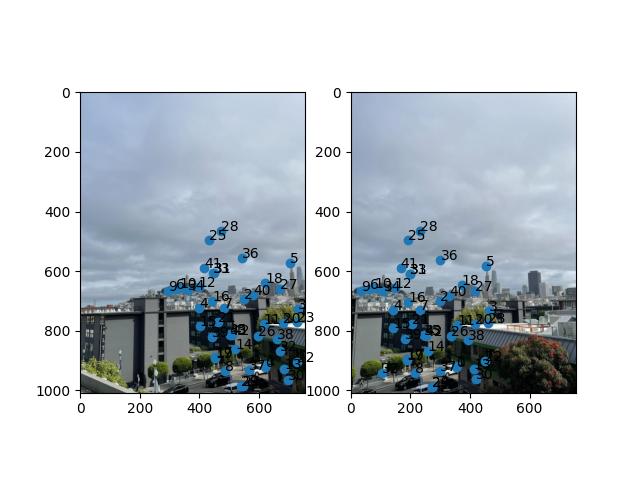
Results
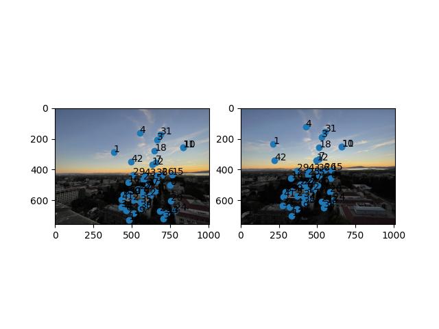
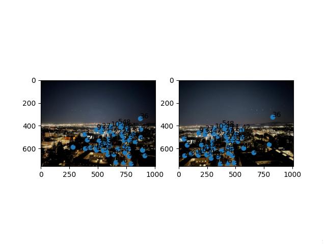
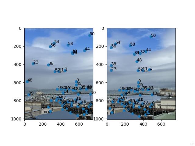
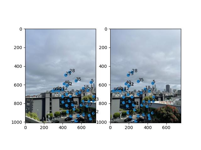
For each of the images below, you can see the matched corners after ANMS for both images.
SF Skyline
Bay Area Sunset
Bay Area Nighttime
United B777 - Bay Fleet Week
RANSAC
Approach
Now that we have matched corners, we want to select the combination of 4 corners which will yield the most accurate homography.
- Choose 4 pairs of corners without replacement at random.
- Compute the homography and map all of the source corners to the target corners through the homography.
- Compare how well these points get mapped by thresholding on the euclidean norm.
- Count how many mapped points are close enough to the original target points.
- Take the max over how many points are “inline" and return the subset of corners that maximizes this value.
This subset of points are the correspondences that will be used to warp images. As a final note, I'm unsure of the exact reason why but RANSAC was a bit “finnicky" with the sunset and nighttime pictures. There seems to be one combination of points that achieves the max inline correspondences but whose homography scales the points way too much. Thus, I always reseeded at the beginning of each call to RANSAC.
Results
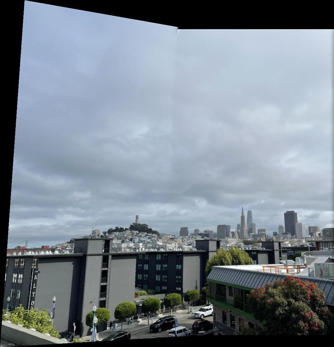
SF Skyline
Bay Area Sunset
Bay Area Nighttime
United B777 - Bay Fleet Week
What I have learned.
I think that the entire formulation on how to find good features and match correspondences is an interesting solution to a difficult problem. I think that the feature matching is one of the more interesting parts of the project; especially the use of Lowe's trick to solve the problem. It is also cool to see that the B777 picture now lines up pretty well even if I didn't employ the best picture taking techniques.
Bells and Whistles
None for this project.